University Foundationscalculustaylor seriesmaclaurin series
infinite sequences and series
Power series represent functions as infinite polynomials, with convergence determining where the representation is valid.
Wed May 06
Infinite Sequences and Series
Objective
Radius and Interval of Convergence
Representations
Differentiation and Integration of Power Series
Taylor Series and Maclaurin Series
1. Power Series
The basic form of a power series is:
n=0∑∞cn(x−a)n
where:
cn are the coefficients;
x is the variable;
a is the center of expansion;
(x−a)n represents powers centered at a.
If a=0, the power series becomes:
n=0∑∞cnxn
This is called a power series centered at 0.
An ordinary polynomial has finitely many terms, for example:
1+x+x2+x3
whereas a power series has infinitely many terms:
1+x+x2+x3+⋯
Many complicated functions can be written in the form of a power series.
For example:
1−x1=1+x+x2+x3+⋯
That is:
1−x1=n=0∑∞xn
2. Radius of Convergence
2.1 What is convergence?
Whether an infinite series is meaningful depends on whether it converges.
For example:
1+21+41+81+⋯
The sum of this series gets closer and closer to 2, so it converges.
However, a series such as:
1+1+1+1+⋯
grows without bound, so it diverges.
2.2 Why do we need to discuss convergence for power series?
A power series contains a variable x. Therefore, for different values of x, the same power series may sometimes converge and sometimes diverge.
For example:
n=0∑∞xn
If x=21:
1+21+41+81+⋯
it converges.
If x=2:
1+2+4+8+⋯
it diverges.
So we need to study:
For which values of x does this power series converge?
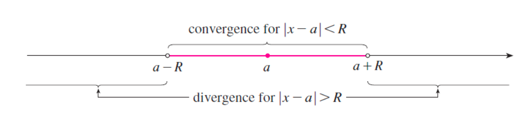
2.3 Radius of convergence R
For the power series:
n=0∑∞cn(x−a)n
there usually exists a number R such that:
when ∣x−a∣<R, the series converges;
when ∣x−a∣>R, the series diverges;
a is the center of convergence.
This number R is called the radius of convergence.
Three cases for R
Case 1: The series converges only at the center
If R=0, this means the series converges only at:
x=a
Case 2: The series converges for all real numbers
If R=∞, this means the series converges for all x.
That is, the interval of convergence is:
(−∞,∞)
Case 3: The series converges near the center
If 0<R<∞, then the series converges when:
∣x−a∣<R
This inequality can be rewritten as:
a−R<x<a+R
So the basic interval of convergence is:
(a−R,a+R)
3. Interval of Convergence
3.1 What is the interval of convergence?
The interval of convergence is the interval consisting of all values of x for which the power series converges.
If the radius of convergence is R and the center is a, then the interior of the interval must be:
(a−R,a+R)
However, the endpoints x=a−R and x=a+R must be checked separately.
Why do the endpoints need to be checked separately?
Because the radius of convergence only tells us that:
the series definitely converges inside the interval;
the series definitely diverges outside the interval.
However, at the endpoints, where ∣x−a∣=R, the series may converge or diverge. Therefore, the endpoints must be substituted back into the original series and checked separately.
Thus, if the center is a and the radius is R, the interval of convergence may be one of the following four possibilities:
(a−R,a+R)(a−R,a+R][a−R,a+R)[a−R,a+R]
In other words:
the left endpoint may or may not be included;
the right endpoint may or may not be included.
4. Geometric Series
The most important starting point is:
1−x1=1+x+x2+x3+⋯
It can also be written as:
1−x1=n=0∑∞xn
This is valid when:
∣x∣<1
Why is this true?
The finite partial sum is:
sn=1+x+x2+⋯+xn
This is the sum of a finite geometric sequence:
sn=1−x1−xn+1
When ∣x∣<1:
xn+1→0
So:
sn→1−x1
Therefore:
1+x+x2+⋯=1−x1
5. Representing Functions Using Geometric Series
The core idea of this section is:
Rewrite the target function into the form 1−r1, and then apply the geometric series formula.
1. Example: Represent 1+x21
We know:
1−x1=n=0∑∞xn
Now we want to represent:
1+x21
Notice that:
1+x2=1−(−x2)
So:
1+x21=1−(−x2)1
Let:
r=−x2
Then:
1+x21=n=0∑∞(−x2)n
Expanding:
1+x21=1−x2+x4−x6+x8−⋯
It can also be written as:
1+x21=n=0∑∞(−1)nx2n
The convergence condition is:
∣−x2∣<1
That is:
x2<1
So:
∣x∣<1
The interval of convergence is:
(−1,1)
2. Example: Represent x+21
We want to rewrite it into the form 1−r1.
First factor out 2 from the denominator:
x+2=2(1+2x)
So:
x+21=2(1+2x)1
That is:
x+21=21⋅1+2x1
Rewrite the plus sign as a minus sign:
1+2x=1−(−2x)
So:
x+21=21⋅1−(−2x)1
Apply the geometric series formula:
1−r1=n=0∑∞rn
Let:
r=−2x
Then:
x+21=21n=0∑∞(−2x)n
Simplifying:
x+21=n=0∑∞2n+1(−1)nxn
The convergence condition is:
−2x<1
So:
2∣x∣<1
That is:
∣x∣<2
The interval of convergence is:
(−2,2)
3. Example: Represent x+2x3
Since we already know that:
x+21=n=0∑∞2n+1(−1)nxn
we have:
x+2x3=x3⋅x+21
Thus:
x+2x3=x3n=0∑∞2n+1(−1)nxn
Multiplying by x3:
x+2x3=n=0∑∞2n+1(−1)nxn+3
Expanding the first few terms:
x+2x3=21x3−41x4+81x5−161x6+⋯
The interval of convergence remains unchanged:
(−2,2)
because multiplying by x3 does not change the convergence condition of the geometric series itself.
6. Term-by-Term Differentiation of Power Series
6.1 Core idea
If a function can be written as a power series:
f(x)=n=0∑∞cn(x−a)n
then inside the interval of convergence, we can differentiate it term by term just like an ordinary polynomial:
f′(x)=n=1∑∞ncn(x−a)n−1
Notice that after differentiation, the sum starts from n=1, because the constant term corresponding to n=0 differentiates to 0.
6.2 Why can we differentiate term by term?
Finite polynomials can certainly be differentiated term by term:
dxd(1+x+x2)=0+1+2x
A power series is like an infinite polynomial.
The theorem tells us that inside the radius of convergence, a power series can also be differentiated term by term.
6.3 Does the radius of convergence change?
Important
After term-by-term differentiation of a power series, the radius of convergence R remains unchanged, but the behavior at the endpoints may change.
In other words:
the original radius is still R;
but whether the endpoints converge needs to be checked again.
Example: Represent (1−x)21
Start from the basic formula:
1−x1=1+x+x2+x3+⋯
That is:
1−x1=n=0∑∞xn
Differentiate both sides.
Left-hand side:
dxd(1−x1)=(1−x)21
Right-hand side:
dxd(1+x+x2+x3+⋯)=1+2x+3x2+4x3+⋯
Therefore:
(1−x)21=1+2x+3x2+4x3+⋯
This can be written as:
(1−x)21=n=1∑∞nxn−1
If we want to write it starting from n=0, we can re-index:
(1−x)21=n=0∑∞(n+1)xn
The radius of convergence is still:
R=1
7. Term-by-Term Integration of Power Series
7.1 Core formula
If:
f(x)=n=0∑∞cn(x−a)n
then:
∫f(x)dx=C+n=0∑∞cnn+1(x−a)n+1
That is, each term can be integrated separately.
Just like differentiation:
After term-by-term integration, the radius of convergence R remains unchanged. However, the endpoints still need to be checked again.
Example: Represent ln(1−x)
We know:
1−x1=1+x+x2+x3+⋯
and:
dxdln(1−x)=−1−x1
So:
−ln(1−x)=∫1−x1dx
Use the series to integrate the right-hand side:
−ln(1−x)=∫(1+x+x2+x3+⋯)dx
Integrating term by term:
−ln(1−x)=x+2x2+3x3+4x4+⋯+C
When x=0:
−ln(1−0)=0
The right-hand side is:
0+C
So:
C=0
Therefore:
−ln(1−x)=x+2x2+3x3+4x4+⋯
Multiplying both sides by −1:
ln(1−x)=−x−2x2−3x3−4x4−⋯
In summation notation:
ln(1−x)=−n=1∑∞nxn
Valid when:
∣x∣<1
Radius of convergence:
R=1
Example: Represent tan−1x
We know:
dxdtan−1x=1+x21
and we have already obtained:
1+x21=1−x2+x4−x6+⋯
So we integrate:
tan−1x=∫1+x21dx
Substitute in the series:
tan−1x=∫(1−x2+x4−x6+⋯)dx
Integrating term by term:
tan−1x=x−3x3+5x5−7x7+⋯
In summation notation:
tan−1x=n=0∑∞(−1)n2n+1x2n+1
Valid when:
∣x∣<1
Radius of convergence:
R=1
8. Using Power Series to Approximate Integrals
8.1 Why use power series to approximate integrals?
Some functions do not have simple elementary antiderivatives.
For example:
∫1+x71dx
This integral is relatively difficult to compute directly.
However, we can write the integrand as a power series and then integrate term by term.
Example: Compute ∫1+x71dx
Rewrite:
1+x71
as:
1−(−x7)1
Applying the geometric series:
1+x71=n=0∑∞(−x7)n
That is:
1+x71=1−x7+x14−x21+⋯
Integrate term by term:
∫1+x71dx=∫(1−x7+x14−x21+⋯)dx
We get:
∫1+x71dx=C+x−8x8+15x15−22x22+⋯
In summation notation:
∫1+x71dx=C+n=0∑∞(−1)n7n+1x7n+1
The convergence condition is:
∣−x7∣<1
That is:
∣x∣<1
If we want to compute:
∫01/21+x71dx
using the antiderivative above and taking C=0:
∫01/21+x71dx=[x−8x8+15x15−22x22+⋯]01/2
Substituting x=21:
=21−8⋅281+15⋅2151−22⋅2221+⋯
This is an alternating series.
If we want to approximate it within a certain error bound, we can use the Alternating Series Estimation Theorem:
For an alternating series, if the absolute values of the terms decrease and tend to 0, then the truncation error is less than the absolute value of the next term.
9. Taylor Series
The core question of Taylor Series
Previously, we obtained power series representations of functions by transforming geometric series.
Now we want to ask a more general question:
Can any function f(x) be written as a power series?
That is, can it be written as:
f(x)=c0+c1(x−a)+c2(x−a)2+c3(x−a)3+⋯
If it can, how should we find the coefficients c0,c1,c2,…?
Suppose:
f(x)=n=0∑∞cn(x−a)n
That is:
f(x)=c0+c1(x−a)+c2(x−a)2+c3(x−a)3+⋯
Finding c0
Let:
x=a
Then:
f(a)=c0+c1(a−a)+c2(a−a)2+⋯
Since:
a−a=0
all terms except the first one become 0.
Therefore:
f(a)=c0
So:
c0=f(a)
Finding c1
Differentiate the original expression:
f′(x)=c1+2c2(x−a)+3c3(x−a)2+4c4(x−a)3+⋯
Let:
x=a
Then:
f′(a)=c1
So:
c1=f′(a)
Finding c2
Differentiate again:
f′′(x)=2c2+3⋅2c3(x−a)+4⋅3c4(x−a)2+⋯
Let x=a:
f′′(a)=2c2
So:
c2=2f′′(a)
That is:
c2=2!f′′(a)
Finding c3
Differentiate once more:
f′′′(a)=3⋅2⋅1c3
So:
f′′′(a)=3!c3
Therefore:
c3=3!f′′′(a)
Continuing in this way, we obtain:
f(n)(a)=n!cn
So:
cn=n!f(n)(a)
This is where the coefficients of the Taylor Series come from.
Comments
No account needed — just leave your name and comment.